ArchGDAL quickstart
This tutorial is highly inspired by the Python Quickstart, and aims to provide a similar introductory guide to the ArchGDAL package.
This guide uses a GeoTIFF image of the band 4 of a Landsat 8 image, covering a part of the United State's Colorado Plateau. This image was acquired on July 12, 2016, and can be download at this link. 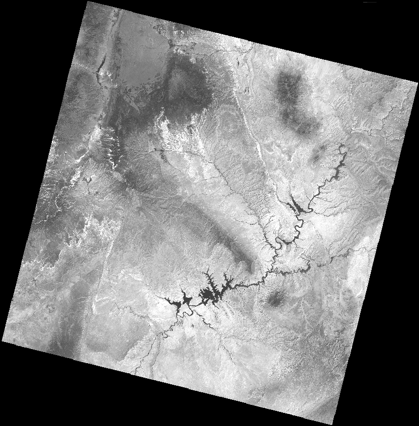
Opening the dataset
Assuming that the ArchGDAL package is already installed, first import the package, and preferably assign an alias to the package.
In this example, we'll be fetching the raster dataset from where it is hosted.
julia> dataset = AG.readraster("/vsicurl/http://landsat-pds.s3.amazonaws.com/c1/L8/037/034/LC08_L1TP_037034_20160712_20170221_01_T1/LC08_L1TP_037034_20160712_20170221_01_T1_B4.TIF")
ERROR: GDALError (CE_Failure, code 11):
	HTTP response code: 403
A dataset can be opened using ArchGDAL's readraster(...) method. This method takes in the path of a dataset as a string, and returns a GDAL Dataset object in read-only mode.
ArchGDAL can read a variety of file types using appropriate drivers. The driver used for opening the dataset can be queried as such.
julia> AG.getdriver(dataset)
ERROR: UndefVarError: `dataset` not defined in `Main.var"ex-quickstart"`
Suggestion: check for spelling errors or missing imports.
Dataset Attributes
A raster dataset can have multiple bands of information. To get the number of bands present in a dataset -
julia> AG.nraster(dataset)
ERROR: UndefVarError: `dataset` not defined in `Main.var"ex-quickstart"`
Suggestion: check for spelling errors or missing imports.
In our case, the raster dataset only has a single band.
Other properties of a raster dataset, such as the width and height can be accessed using the following functions
julia> AG.width(dataset)
ERROR: UndefVarError: `dataset` not defined in `Main.var"ex-quickstart"`
Suggestion: check for spelling errors or missing imports.

julia> AG.height(dataset)
ERROR: UndefVarError: `dataset` not defined in `Main.var"ex-quickstart"`
Suggestion: check for spelling errors or missing imports.
Dataset Georeferencing
All raster datasets contain embedded georeferencing information, using which the raster image can be located at a geographic location. The georeferencing attributes are stored as the dataset's Geospatial Transform.
julia> gt = AG.getgeotransform(dataset)
ERROR: UndefVarError: `dataset` not defined in `Main.var"ex-quickstart"`
Suggestion: check for spelling errors or missing imports.
The x-y coordinates of the top-left corner of the raster dataset are denoted by gt[1] and gt[4] values. In this case, the coordinates . The cell size is represented by gt[2] and gt[6] values, corresponding to the cell size in x and y directions respectively, and the gt[3] and gt[5] values define the rotation. In our case, the top left pixel is at an offset of 358485.0m and 4.265115e6m in x and y directions respectively, from the origin.
The Origin of the dataset is defined using what is called, a Coordinate Reference System (CRS in short).
julia> p = AG.getproj(dataset)
ERROR: UndefVarError: `dataset` not defined in `Main.var"ex-quickstart"`
Suggestion: check for spelling errors or missing imports.
The getproj(...) function returns the projection of a dataset as a string representing the CRS in the OpenGIS WKT format. To convert it into other CRS representations, such as PROJ.4, toPROJ4(...) can be used. However, first the string representation of the CRS has to be converted into an ArchGDAL.ISpatialRef type using the importWKT(...) function.
julia> AG.toPROJ4(AG.importWKT(p))
ERROR: UndefVarError: `p` not defined in `Main.var"ex-quickstart"`
Suggestion: check for spelling errors or missing imports.
Reading Raster data
In the previous steps, we read the raster file as a dataset. To obtain the actual raster data, we can slice the array accordingly.
julia> dataset[:, :, 1]
ERROR: UndefVarError: `dataset` not defined in `Main.var"ex-quickstart"`
Suggestion: check for spelling errors or missing imports.
Since the dimensions of the dataset are [cols, rows, bands], respectively, using [:, :, 1] returns all the columns and rows for the first band. Accordingly other complex slice operations can also be performed.
To get the individual band
julia> band = AG.getband(dataset, 1)
ERROR: UndefVarError: `dataset` not defined in `Main.var"ex-quickstart"`
Suggestion: check for spelling errors or missing imports.
Band specific attributes can be easily accessed through a variety of functions
julia> AG.width(band)
ERROR: UndefVarError: `band` not defined in `Main.var"ex-quickstart"`
Suggestion: check for spelling errors or missing imports.

julia> AG.height(band)
ERROR: UndefVarError: `band` not defined in `Main.var"ex-quickstart"`
Suggestion: check for spelling errors or missing imports.

julia> AG.getnodatavalue(band)
ERROR: UndefVarError: `band` not defined in `Main.var"ex-quickstart"`
Suggestion: check for spelling errors or missing imports.

julia> AG.indexof(band)
ERROR: UndefVarError: `band` not defined in `Main.var"ex-quickstart"`
Suggestion: check for spelling errors or missing imports.
The no-data value of the band can be obtained using the getnodatavalue(...) function, which in our case is -1.0e10.
Writing into Dataset
Creating dummy data to be written as raster dataset.
x = range(-4.0, 4.0, length=240)
y = range(-3.0, 3.0, length=180)
X = repeat(collect(x)', size(y)[1])
Y = repeat(collect(y), 1, size(x)[1])
Z1 = exp.(-2*log(2) .*((X.-0.5).^2 + (Y.-0.5).^2)./(1^2))
Z2 = exp.(-3*log(2) .*((X.+0.5).^2 + (Y.+0.5).^2)./(2.5^2))
Z = 10.0 .* (Z2 .- Z1)
180×240 Matrix{Float64}:
0.0212253 0.0229376 0.0247696 0.026728 … 0.00163782 0.00148217
0.0224341 0.0242439 0.0261802 0.0282501 0.00173109 0.00156658
0.023694 0.0256055 0.0276505 0.0298367 0.00182831 0.00165456
0.0250059 0.0270233 0.0291816 0.0314888 0.00192955 0.00174618
0.0263708 0.0284983 0.0307744 0.0332075 0.00203487 0.00184149
0.0277894 0.0300313 0.0324298 0.0349939 … 0.00214433 0.00194055
0.0292625 0.0316232 0.0341488 0.0368488 0.002258 0.00204341
0.0307905 0.0332745 0.0359321 0.038773 0.00237591 0.00215012
0.0323742 0.0349859 0.0377802 0.0407672 0.00249811 0.0022607
0.0340139 0.0367579 0.0396937 0.042832 0.00262463 0.0023752
⋮ ⋱
0.00525686 0.00568095 0.00613468 0.00661971 0.000405638 0.000367089
0.00488943 0.00528388 0.00570589 0.00615702 0.000377286 0.000341431
0.00454428 0.00491088 0.00530311 0.00572239 0.000350653 0.000317329
0.00422034 0.00456081 0.00492507 0.00531446 0.000325656 0.000294708
0.00391656 0.00423252 0.00457056 0.00493193 … 0.000302216 0.000273495
0.00363193 0.00392493 0.00423841 0.00457351 0.000280253 0.000253619
0.00336547 0.00363697 0.00392745 0.00423797 0.000259691 0.000235012
0.00311622 0.00336762 0.00363659 0.00392411 0.000240459 0.000217607
0.00288328 0.00311589 0.00336475 0.00363078 0.000222484 0.000201341The fictional field for this example consists of the difference of two Gaussian distributions and is represented by the array Z. Its contours are shown below. 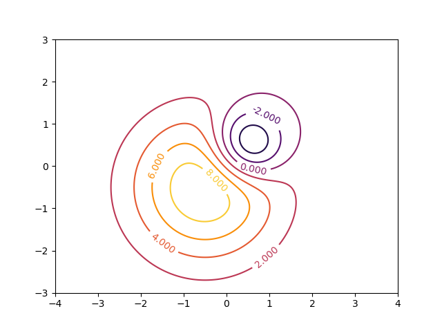
Once we have the data to write into a raster dataset, before performing the write operation itself, it is a good idea to define the geotransform and the coordinate reference system of the resulting dataset. For North-up raster images, only the pixel-size/resolution and the coordinates of the upper-left pixel is required.
# Resolution
res = (x[end] - x[1]) /240.0

# Upper-left pixel coordinates
ul_x = x[1] - res/2
ul_y = y[1] - res/2

gt = [ul_x, res, 0.0, ul_y, 0.0, res]
6-element Vector{Float64}:
-4.016666666666667
0.03333333333333333
0.0
-3.0166666666666666
0.0
0.03333333333333333The coordinate reference system of the dataset needs to be a string in the WKT format.
crs = AG.toWKT(AG.importPROJ4("+proj=latlong"))"GEOGCS[\"unknown\",DATUM[\"WGS_1984\",SPHEROID[\"WGS 84\",6378137,298.257223563,AUTHORITY[\"EPSG\",\"7030\"]],AUTHORITY[\"EPSG\",\"6326\"]],PRIMEM[\"Greenwich\",0,AUTHORITY[\"EPSG\",\"8901\"]],UNIT[\"degree\",0.0174532925199433,AUTHORITY[\"EPSG\",\"9122\"]],AXIS[\"Longitude\",EAST],AXIS[\"Latitude\",NORTH]]"
To write this array, first a dataset has to be created. This can be done using the AG.create function. The first argument defines the path of the resulting dataset. The following keyword arguments are hopefully self-explanatory.
Once inside the do...end block, the write! method can be used to write the array(Z), in the 1st band of the opened dataset. Next, the geotransform and CRS can be specified using the setgeotransform! and setproj! methods.
AG.create(
    "./temporary.tif",
    driver = AG.getdriver("GTiff"),
    width=240,
    height=180,
    nbands=1,
    dtype=Float64
) do dataset
    AG.write!(dataset, Z, 1)

    AG.setgeotransform!(dataset, gt)
    AG.setproj!(dataset, crs)
end
NULL Dataset